Análisis de similitud estructural entre moléculas pequeñas usando la similitud de Tanimoto.
Este script de Python es una herramienta integral para el análisis de similitud y el agrupamiento jerárquico de moléculas basado en sus estructuras químicas.
Sus principales utilidades son:
- Cálculo de similitud molecular: el script toma como entrada moléculas representadas por sus cadenas SMILES (Simplified Molecular Input Line Entry System). Convierte estas moléculas en huellas dactilares moleculares (Morgan fingerprints), que son representaciones numéricas de su estructura. Luego, calcula una matriz de distancia basada en la similitud de Tanimoto entre todas las parejas de moléculas. La similitud de Tanimoto es una métrica estándar para cuantificar cuán similares son dos moléculas estructuralmente.
- Agrupamiento jerárquico aglomerativo: aplica el algoritmo de agrupamiento jerárquico aglomerativo para organizar las moléculas en grupos (clusters) basándose en su similitud estructural. Esto permite identificar subconjuntos de moléculas que comparten características estructurales similares. El script realiza este agrupamiento utilizando diferentes umbrales de similitud (90%, 80% y 70%), lo que permite explorar la agrupación a diferentes niveles de granularidad.
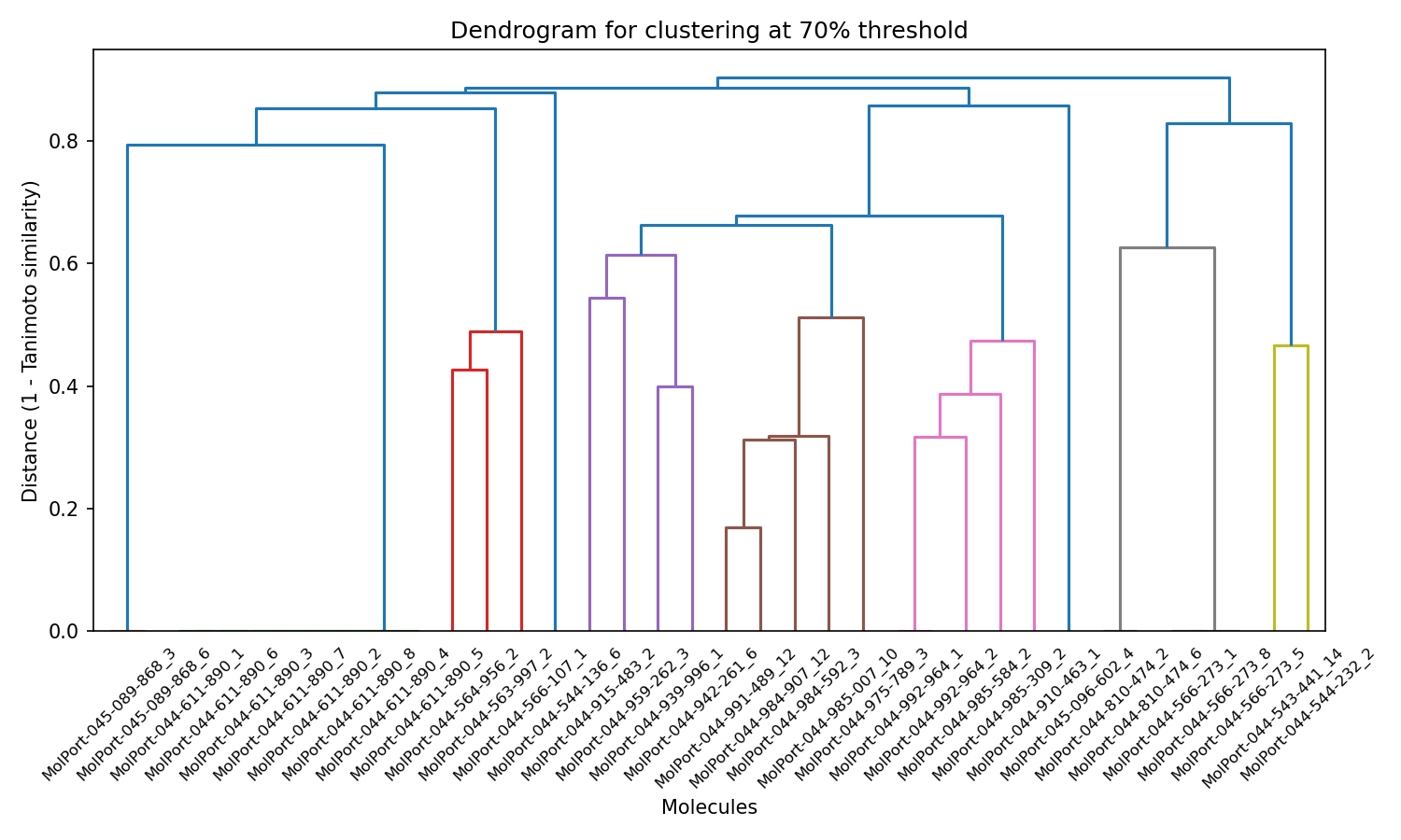
- Visualización de agrupamientos mediante dendrogramas: para cada umbral de similitud, el script genera un dendrograma. Un dendrograma es un diagrama en forma de árbol que ilustra las relaciones jerárquicas entre los grupos. Permite visualizar cómo las moléculas se agrupan progresivamente a medida que disminuye el umbral de similitud, facilitando la interpretación de los resultados del agrupamiento.
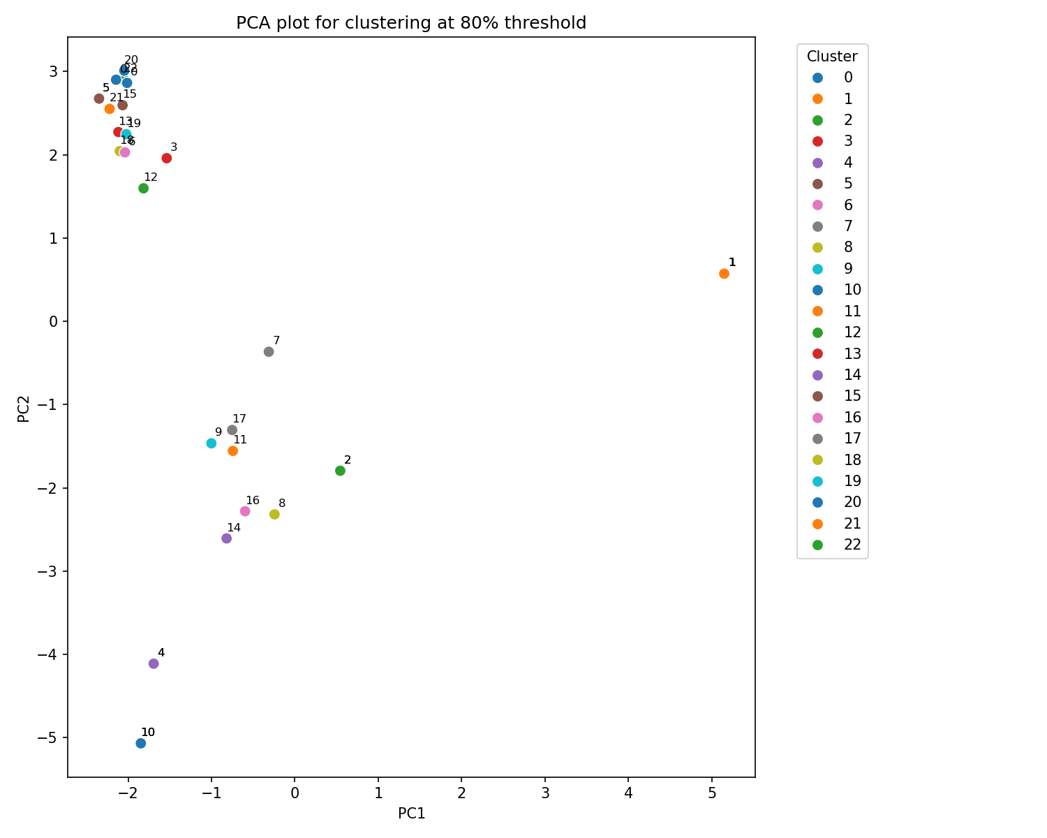
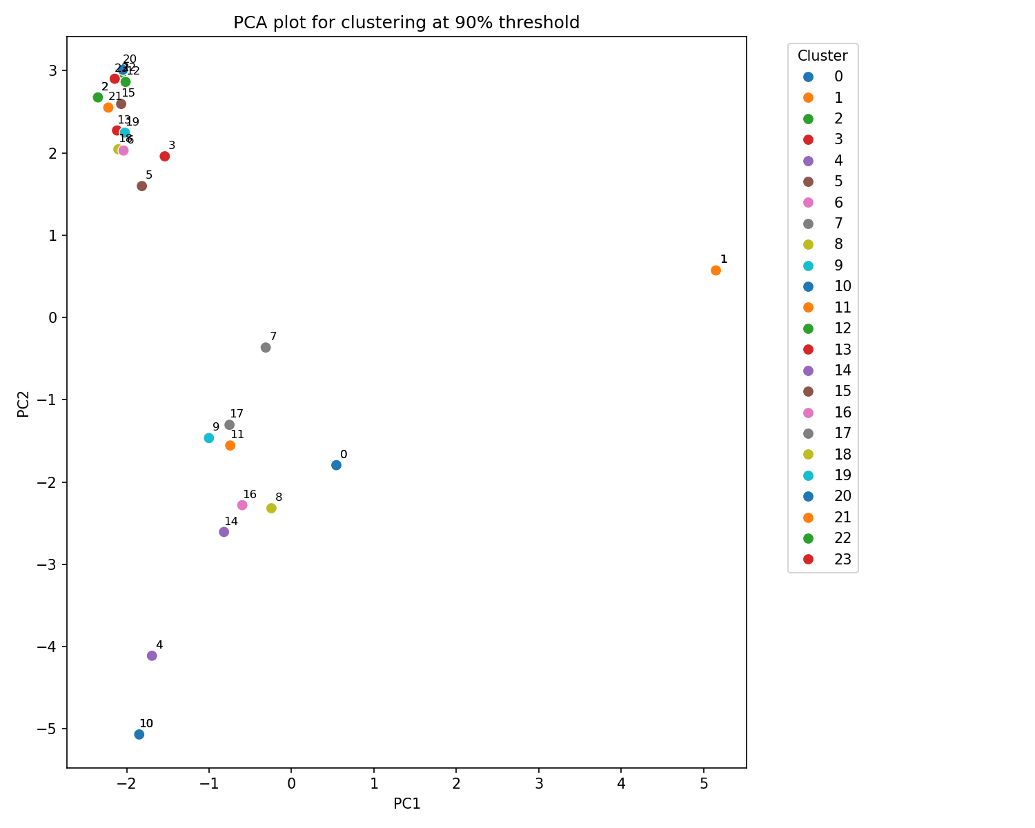
- Reducción de dimensionalidad y visualización con PCA: utiliza el Análisis de Componentes Principales (PCA) para reducir la dimensionalidad de los datos de las huellas dactilares moleculares a dos componentes principales. Luego, crea un gráfico de dispersión donde cada punto representa una molécula, coloreado según el grupo al que pertenece en el agrupamiento. Esta visualización permite observar la distribución de las moléculas en un espacio 2D y cómo se separan o agrupan visualmente.
- Los resultados del agrupamiento, incluyendo las etiquetas de los clusters para cada molécula, se guardan en archivos de texto separados para cada umbral de similitud. Además, los dendrogramas y los gráficos PCA se guardan como imágenes (archivos PNG).
Para ejecutar el script de Python que tienes justo debajo, necesitarás tener instalados los siguientes módulos en tu entorno. Puedes instalarlos fácilmente usando pip, el gestor de paquetes de Python, o bien con conda.
pip install pandas rdkit scikit-learn numpy matplotlib seaborn scipy  # pip
conda install -c conda-forge pandas scikit-learn numpy matplotlib seaborn scipy rdkit  # conda
import pandas as pd
from rdkit import Chem
from rdkit.Chem import DataStructs
from rdkit.Chem.rdFingerprintGenerator import GetMorganGenerator
from sklearn.cluster import AgglomerativeClustering
from sklearn.decomposition import PCA
import numpy as np
import matplotlib.pyplot as plt
import seaborn as sns
from scipy.cluster.hierarchy import linkage, dendrogram
from scipy.spatial.distance import squareform
import os
# File paths
input_file = r'd:\zzz\_moleculas.txt'
output_folder = r'd:\zzz'
os.makedirs(output_folder, exist_ok=True)
# Read input file
df = pd.read_csv(input_file, sep='\t')
names = df.iloc[:, 0].tolist()
smiles = df.iloc[:, 1].tolist()
# Convert SMILES to molecules and fingerprints using MorganGenerator
mol_list = [Chem.MolFromSmiles(s) for s in smiles]
generator = GetMorganGenerator(radius=2, fpSize=2048)
fps = [generator.GetFingerprint(m) for m in mol_list]
# Function to calculate distance matrix based on Tanimoto similarity
def calc_distance_matrix(fps):
n = len(fps)
dist_mat = np.zeros((n, n))
for i in range(n):
for j in range(i + 1, n):
sim = DataStructs.TanimotoSimilarity(fps[i], fps[j])
dist_mat[i, j] = 1 - sim
dist_mat[j, i] = dist_mat[i, j]
return dist_mat
distance_matrix = calc_distance_matrix(fps)
# Similarity thresholds
thresholds = [0.9, 0.8, 0.7]
for threshold in thresholds:
distance_threshold = 1 - threshold
# Hierarchical clustering with precomputed distance matrix
clustering = AgglomerativeClustering(
metric='precomputed',
linkage='complete',
distance_threshold=distance_threshold,
n_clusters=None
)
cluster_labels = clustering.fit_predict(distance_matrix)
# Save clusters to file
df_out = df.copy()
df_out[f'Cluster_{int(threshold * 100)}'] = cluster_labels
output_clusters = os.path.join(output_folder, f'clusters_{int(threshold * 100)}.txt')
df_out.to_csv(output_clusters, sep='\t', index=False)
print(f'Clusters with threshold {int(threshold * 100)}% saved to: {output_clusters}')
# Convert full distance matrix to condensed format for linkage
condensed_dist_matrix = squareform(distance_matrix)
# Generate dendrogram
linked = linkage(condensed_dist_matrix, method='complete')
plt.figure(figsize=(10, 6))
dendrogram(linked, labels=names, orientation='top', distance_sort='descending', show_leaf_counts=True)
plt.title(f'Dendrogram for clustering at {int(threshold * 100)}% threshold')
plt.xlabel('Molecules')
plt.ylabel('Distance (1 - Tanimoto similarity)')
plt.tight_layout()
dendrogram_file = os.path.join(output_folder, f'dendrogram_{int(threshold * 100)}.png')
plt.savefig(dendrogram_file, dpi=150)
plt.close()
print(f'Dendrogram saved to: {dendrogram_file}')
# Perform PCA on fingerprint bits (convert to numpy array)
fps_array = np.array([list(fp) for fp in fps], dtype=int)
pca = PCA(n_components=2)
coords = pca.fit_transform(fps_array)
# Plot PCA scatter colored by cluster
plt.figure(figsize=(10, 8)) # Aumentamos el tamaño para mejor visualización de las etiquetas
palette = sns.color_palette("tab10", np.unique(cluster_labels).max() + 1)
sns.scatterplot(x=coords[:, 0], y=coords[:, 1], hue=cluster_labels, palette=palette, legend='full', s=60)
# --- INICIO DE LA MODIFICACIÓN PARA AÑADIR LAS ETIQUETAS DE CLÚSTER ---
for i, txt in enumerate(cluster_labels):
plt.annotate(txt, (coords[i, 0], coords[i, 1]), textcoords="offset points", xytext=(5,5), ha='center', fontsize=8)
# --- FIN DE LA MODIFICACIÓN ---
plt.title(f'PCA plot for clustering at {int(threshold * 100)}% threshold')
plt.xlabel('PC1')
plt.ylabel('PC2')
plt.legend(title='Cluster', bbox_to_anchor=(1.05, 1), loc='upper left')
plt.tight_layout(rect=[0, 0, 0.85, 1]) # leave some room on right for legend
pca_file = os.path.join(output_folder, f'pca_{int(threshold * 100)}.png')
plt.savefig(pca_file, dpi=150)
plt.close()
print(f'PCA plot saved to: {pca_file}')Los datos de partida se encuentran en el fichero _moleculas.txt, en la ruta d:\zzz\. Cambia estos parámetros según tus necesidades.
Name	SMILES
MolPort-044-984-592_3	OC(=O)[C@@H]1OCC[C@H]1NC(=O)[C@@H]1OCC[C@@H]1CNC(=O)OCC1c2c(cccc2)c2c1cccc2
MolPort-044-985-007_10	OC(=O)[C@H]1OCC[C@@H]1CNC(=O)[C@@H]1COC[C@H]1NC(=O)OCC1c2c(cccc2)c2c1cccc2
MolPort-044-566-107_1	O=C(NCCN1C[C@@H]2C[C@H](C1)c1cccc(=O)n1C2)c1n[nH]c(c1)c1cc2c(OCC2)cc1
MolPort-044-984-907_12	OC(=O)[C@H]1OCC[C@H]1CNC(=O)[C@@H]1OCC[C@H]1NC(=O)OCC1c2c(cccc2)c2c1cccc2
MolPort-044-942-261_6	OC(=O)[C@H]1CN(CCO1)C(=O)[C@@H]1C[C@@H](NC(=O)OCC2c3c(cccc3)c3c2cccc3)C=C1
MolPort-044-975-789_3	OC(=O)Cn1cc(NC(=O)[C@@H]2OCC[C@H]2NC(=O)OCC2c3c(cccc3)c3c2cccc3)cn1
MolPort-044-991-489_12	OC(=O)[C@H]1C[C@H]1CNC(=O)[C@@H]1OCC[C@H]1NC(=O)OCC1c2c(cccc2)c2c1cccc2
MolPort-044-992-964_2	OC(=O)[C@H]1CN(CC21CC2)C(=O)C#CCNC(=O)OCC1c2c(cccc2)c2c1cccc2
MolPort-044-563-997_2	COc1c(cccc1)c1n[nH]c(c1)C(=O)NCCN1C[C@H]2C[C@H](C1)c1cccc(=O)n1C2
MolPort-044-985-584_2	C[C@H]1CN(C[C@@H]1C(=O)O)C(=O)C#CCNC(=O)OCC1c2c(cccc2)c2c1cccc2
MolPort-044-992-964_1	OC(=O)[C@@H]1CN(CC21CC2)C(=O)C#CCNC(=O)OCC1c2c(cccc2)c2c1cccc2
MolPort-044-544-232_2	COc1nn2c(CCCC(=O)N3CCCC4=C[C@@H]5C[C@@H](CN6CCCC[C@H]56)[C@H]34)nnc2cc1
MolPort-044-910-463_1	OC(=O)[C@]12CN(C[C@@H]1COCC2)C(=O)C#CCNC(=O)OCC1c2c(cccc2)c2c1cccc2
MolPort-044-543-441_14	O=C(CCCn1nnc2ccccc2c1=O)N1CCCC2=C[C@H]3C[C@H](CN4CCCC[C@@H]34)[C@@H]12
MolPort-044-985-309_2	OC(=O)[C@H]1[C@H]2C[C@@H]1N(C2)C(=O)C#CCNC(=O)OCC1c2c(cccc2)c2c1cccc2
MolPort-044-810-474_6	CC1(C)CC(=O)c2c(O)cc(OCC(=O)N3C[C@H]4C[C@H](C3)[C@H]3CCCC(=O)N3C4)cc2O1
MolPort-044-810-474_2	CC1(C)CC(=O)c2c(O)cc(OCC(=O)N3C[C@H]4C[C@H](C3)[C@@H]3CCCC(=O)N3C4)cc2O1
MolPort-044-611-890_6	C[C@@H](NC(=O)NC[C@@H]1C[C@@H](CO1)c1ccccc1)c1nnnn1c1ccccc1
MolPort-044-611-890_1	C[C@H](NC(=O)NC[C@@H]1C[C@H](CO1)c1ccccc1)c1nnnn1c1ccccc1
MolPort-044-611-890_3	C[C@H](NC(=O)NC[C@H]1C[C@H](CO1)c1ccccc1)c1nnnn1c1ccccc1
MolPort-044-611-890_7	C[C@H](NC(=O)NC[C@H]1C[C@@H](CO1)c1ccccc1)c1nnnn1c1ccccc1
MolPort-044-611-890_2	C[C@@H](NC(=O)NC[C@@H]1C[C@H](CO1)c1ccccc1)c1nnnn1c1ccccc1
MolPort-044-611-890_8	C[C@@H](NC(=O)NC[C@H]1C[C@@H](CO1)c1ccccc1)c1nnnn1c1ccccc1
MolPort-044-611-890_4	C[C@@H](NC(=O)NC[C@H]1C[C@H](CO1)c1ccccc1)c1nnnn1c1ccccc1
MolPort-044-564-956_2	O=C(NCCN1C[C@H]2C[C@H](C1)c1cccc(=O)n1C2)c1c2COc3ccccc3c2n[nH]1
MolPort-044-611-890_5	C[C@H](NC(=O)NC[C@@H]1C[C@@H](CO1)c1ccccc1)c1nnnn1c1ccccc1
MolPort-044-544-136_6	COc1c2C(=O)[C@@]3(Oc2c(Cl)c(OC)c1)[C@H](C)CC(=CC3=O)N[C@@H](Cc1ccccc1)C(=O)N
MolPort-044-959-262_3	OC(=O)[C@@H]1[C@@H]2C[C@H]1N(C2)C(=O)c1nonc1NC(=O)OCC1c2c(cccc2)c2c1cccc2
MolPort-045-096-602_4	N[C@H]1CC[C@H]2CN(C[C@H]12)C(=O)C1CCN(CC1)C(=O)c1cccc2ccccc12
MolPort-044-915-483_2	OC(=O)[C@H]1COCCN1C(=O)c1noc(NC(=O)OCC2c3c(cccc3)c3c2cccc3)c1
MolPort-044-566-273_8	[C@H]12CN(C[C@@H](C1)[C@H]1CCCC(=O)N1C2)C(=O)c1c([nH]nc1)c1cc2c(OCCO2)cc1
MolPort-044-939-996_1	OC(=O)[C@@H]1CN(CCO1)C(=O)C1(CCC1)NC(=O)OCC1c2c(cccc2)c2c1cccc2
MolPort-044-566-273_1	[C@@H]12CN(C[C@H](C1)[C@@H]1CCCC(=O)N1C2)C(=O)c1c([nH]nc1)c1cc2c(OCCO2)cc1
MolPort-044-566-273_5	[C@@H]12CN(C[C@H](C1)[C@H]1CCCC(=O)N1C2)C(=O)c1c([nH]nc1)c1cc2c(OCCO2)cc1
MolPort-045-089-868_6	Cc1c(nnn1c1cccc(c1)[N+](=O)[O-])C(=O)N[C@H]1[C@@H]2CCC[C@H]1C[C@H](N)C2
MolPort-045-089-868_3	Cc1c(nnn1c1cccc(c1)[N+](=O)[O-])C(=O)N[C@@H]1[C@H]2CCC[C@@H]1C[C@H](N)C2
Se generarán tres ficheros de texto con los agrupamientos: clusters_70.txt, clusters_80.txt y clusters_90.txt. En un mismo fichero de texto: clusters_70_80_90.txt. También tres dendrogramas que ves justo debajo.


También se generan tres gráficos PCA que ves justo debajo.

Valores de pertenencia de cada compuesto a un número de cluster en función del grado de similitud.
| Name | SMILES | Cluster_70 | Cluster_80 | Cluster_90 |
|---|---|---|---|---|
| MolPort-044-984-592_3 | OC(=O)[C@@H]1OCC[C@H]1NC(=O)[C@@H]1OCC[C@@H]1CNC(=O)OCC1c2c(cccc2)c2c1cccc2 | 22 | 22 | 22 |
| MolPort-044-985-007_10 | OC(=O)[C@H]1OCC[C@@H]1CNC(=O)[C@@H]1COC[C@H]1NC(=O)OCC1c2c(cccc2)c2c1cccc2 | 20 | 20 | 20 |
| MolPort-044-566-107_1 | O=C(NCCN1C[C@@H]2C[C@H](C1)c1cccc(=O)n1C2)c1n[nH]c(c1)c1cc2c(OCC2)cc1 | 14 | 14 | 14 |
| MolPort-044-984-907_12 | OC(=O)[C@H]1OCC[C@H]1CNC(=O)[C@@H]1OCC[C@H]1NC(=O)OCC1c2c(cccc2)c2c1cccc2 | 0 | 0 | 23 |
| MolPort-044-942-261_6 | OC(=O)[C@H]1CN(CCO1)C(=O)[C@@H]1C[C@@H](NC(=O)OCC2c3c(cccc3)c3c2cccc3)C=C1 | 18 | 18 | 18 |
| MolPort-044-975-789_3 | OC(=O)Cn1cc(NC(=O)[C@@H]2OCC[C@H]2NC(=O)OCC2c3c(cccc3)c3c2cccc3)cn1 | 13 | 13 | 13 |
| MolPort-044-991-489_12 | OC(=O)[C@H]1C[C@H]1CNC(=O)[C@@H]1OCC[C@H]1NC(=O)OCC1c2c(cccc2)c2c1cccc2 | 0 | 0 | 12 |
| MolPort-044-992-964_2 | OC(=O)[C@H]1CN(CC21CC2)C(=O)C#CCNC(=O)OCC1c2c(cccc2)c2c1cccc2 | 5 | 5 | 2 |
| MolPort-044-563-997_2 | COc1c(cccc1)c1n[nH]c(c1)C(=O)NCCN1C[C@H]2C[C@H](C1)c1cccc(=O)n1C2 | 17 | 17 | 17 |
| MolPort-044-985-584_2 | C[C@H]1CN(C[C@@H]1C(=O)O)C(=O)C#CCNC(=O)OCC1c2c(cccc2)c2c1cccc2 | 21 | 21 | 21 |
| MolPort-044-992-964_1 | OC(=O)[C@@H]1CN(CC21CC2)C(=O)C#CCNC(=O)OCC1c2c(cccc2)c2c1cccc2 | 5 | 5 | 2 |
| MolPort-044-544-232_2 | COc1nn2c(CCCC(=O)N3CCCC4=C[C@@H]5C[C@@H](CN6CCCC[C@H]56)[C@H]34)nnc2cc1 | 16 | 16 | 16 |
| MolPort-044-910-463_1 | OC(=O)[C@]12CN(C[C@@H]1COCC2)C(=O)C#CCNC(=O)OCC1c2c(cccc2)c2c1cccc2 | 15 | 15 | 15 |
| MolPort-044-543-441_14 | O=C(CCCn1nnc2ccccc2c1=O)N1CCCC2=C[C@H]3C[C@H](CN4CCCC[C@@H]34)[C@@H]12 | 8 | 8 | 8 |
| MolPort-044-985-309_2 | OC(=O)[C@H]1[C@H]2C[C@@H]1N(C2)C(=O)C#CCNC(=O)OCC1c2c(cccc2)c2c1cccc2 | 19 | 19 | 19 |
| MolPort-044-810-474_6 | CC1(C)CC(=O)c2c(O)cc(OCC(=O)N3C[C@H]4C[C@H](C3)[C@H]3CCCC(=O)N3C4)cc2O1 | 4 | 4 | 4 |
| MolPort-044-810-474_2 | CC1(C)CC(=O)c2c(O)cc(OCC(=O)N3C[C@H]4C[C@H](C3)[C@@H]3CCCC(=O)N3C4)cc2O1 | 4 | 4 | 4 |
| MolPort-044-611-890_6 | C[C@@H](NC(=O)NC[C@@H]1C[C@@H](CO1)c1ccccc1)c1nnnn1c1ccccc1 | 1 | 1 | 1 |
| MolPort-044-611-890_1 | C[C@H](NC(=O)NC[C@@H]1C[C@H](CO1)c1ccccc1)c1nnnn1c1ccccc1 | 1 | 1 | 1 |
| MolPort-044-611-890_3 | C[C@H](NC(=O)NC[C@H]1C[C@H](CO1)c1ccccc1)c1nnnn1c1ccccc1 | 1 | 1 | 1 |
| MolPort-044-611-890_7 | C[C@H](NC(=O)NC[C@H]1C[C@@H](CO1)c1ccccc1)c1nnnn1c1ccccc1 | 1 | 1 | 1 |
| MolPort-044-611-890_2 | C[C@@H](NC(=O)NC[C@@H]1C[C@H](CO1)c1ccccc1)c1nnnn1c1ccccc1 | 1 | 1 | 1 |
| MolPort-044-611-890_8 | C[C@@H](NC(=O)NC[C@H]1C[C@@H](CO1)c1ccccc1)c1nnnn1c1ccccc1 | 1 | 1 | 1 |
| MolPort-044-611-890_4 | C[C@@H](NC(=O)NC[C@H]1C[C@H](CO1)c1ccccc1)c1nnnn1c1ccccc1 | 1 | 1 | 1 |
| MolPort-044-564-956_2 | O=C(NCCN1C[C@H]2C[C@H](C1)c1cccc(=O)n1C2)c1c2COc3ccccc3c2n[nH]1 | 11 | 11 | 11 |
| MolPort-044-611-890_5 | C[C@H](NC(=O)NC[C@@H]1C[C@@H](CO1)c1ccccc1)c1nnnn1c1ccccc1 | 1 | 1 | 1 |
| MolPort-044-544-136_6 | COc1c2C(=O)[C@@]3(Oc2c(Cl)c(OC)c1)[C@H](C)CC(=CC3=O)N[C@@H](Cc1ccccc1)C(=O)N | 7 | 7 | 7 |
| MolPort-044-959-262_3 | OC(=O)[C@@H]1[C@@H]2C[C@H]1N(C2)C(=O)c1nonc1NC(=O)OCC1c2c(cccc2)c2c1cccc2 | 12 | 12 | 5 |
| MolPort-045-096-602_4 | N[C@H]1CC[C@H]2CN(C[C@H]12)C(=O)C1CCN(CC1)C(=O)c1cccc2ccccc12 | 9 | 9 | 9 |
| MolPort-044-915-483_2 | OC(=O)[C@H]1COCCN1C(=O)c1noc(NC(=O)OCC2c3c(cccc3)c3c2cccc3)c1 | 3 | 3 | 3 |
| MolPort-044-566-273_8 | [C@H]12CN(C[C@@H](C1)[C@H]1CCCC(=O)N1C2)C(=O)c1c([nH]nc1)c1cc2c(OCCO2)cc1 | 10 | 10 | 10 |
| MolPort-044-939-996_1 | OC(=O)[C@@H]1CN(CCO1)C(=O)C1(CCC1)NC(=O)OCC1c2c(cccc2)c2c1cccc2 | 6 | 6 | 6 |
| MolPort-044-566-273_1 | [C@@H]12CN(C[C@H](C1)[C@@H]1CCCC(=O)N1C2)C(=O)c1c([nH]nc1)c1cc2c(OCCO2)cc1 | 10 | 10 | 10 |
| MolPort-044-566-273_5 | [C@@H]12CN(C[C@H](C1)[C@H]1CCCC(=O)N1C2)C(=O)c1c([nH]nc1)c1cc2c(OCCO2)cc1 | 10 | 10 | 10 |
| MolPort-045-089-868_6 | Cc1c(nnn1c1cccc(c1)[N+](=O)[O-])C(=O)N[C@H]1[C@@H]2CCC[C@H]1C[C@H](N)C2 | 2 | 2 | 0 |
| MolPort-045-089-868_3 | Cc1c(nnn1c1cccc(c1)[N+](=O)[O-])C(=O)N[C@@H]1[C@H]2CCC[C@@H]1C[C@H](N)C2 | 2 | 2 | 0 |
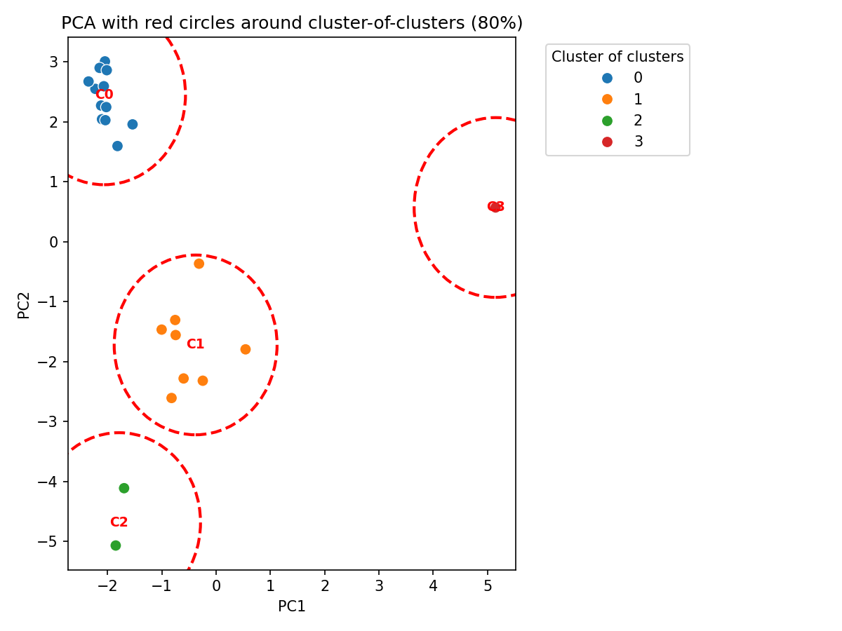
Una nueva versión del script anterior generar "clusters de clusters", o sea, agrupa aquellos clusters que en los gráficos PCA se encuentran dentro de un área de circunferencia correspondiente a 1.5 unidades PCA como radio. Además genera ficcheros de texto para cada grado de identidad (70%, 80% y 90%) que incluyen los nombres de las moléculas que pertenecen a cada supercluster.
import pandas as pd
from rdkit import Chem
from rdkit.Chem import DataStructs
from rdkit.Chem.rdFingerprintGenerator import GetMorganGenerator
from sklearn.cluster import AgglomerativeClustering, DBSCAN
from sklearn.decomposition import PCA
import numpy as np
import matplotlib.pyplot as plt
import seaborn as sns
from scipy.cluster.hierarchy import linkage, dendrogram
from scipy.spatial.distance import squareform
import os

# Input and output
input_file = r'd:\zzz\_buenos.txt'
output_folder = r'd:\zzz'
os.makedirs(output_folder, exist_ok=True)

# Load input
df = pd.read_csv(input_file, sep='\t')
names = df.iloc[:, 0].tolist()
smiles = df.iloc[:, 1].tolist()

# Generate fingerprints
mol_list = [Chem.MolFromSmiles(s) for s in smiles]
generator = GetMorganGenerator(radius=2, fpSize=2048)
fps = [generator.GetFingerprint(m) for m in mol_list]

# Tanimoto distance matrix
def calc_distance_matrix(fps):
    n = len(fps)
    dist_mat = np.zeros((n, n))
    for i in range(n):
        for j in range(i + 1, n):
            sim = DataStructs.TanimotoSimilarity(fps[i], fps[j])
            dist = 1 - sim
            dist_mat[i, j] = dist
            dist_mat[j, i] = dist
    return dist_mat

distance_matrix = calc_distance_matrix(fps)

# Loop over thresholds
thresholds = [0.9, 0.8, 0.7]
for threshold in thresholds:
    distance_threshold = 1 - threshold

    # Hierarchical clustering
    clustering = AgglomerativeClustering(
        metric='precomputed',
        linkage='complete',
        distance_threshold=distance_threshold,
        n_clusters=None
    )
    cluster_labels = clustering.fit_predict(distance_matrix)

    # Save cluster assignments
    df_out = df.copy()
    df_out[f'Cluster_{int(threshold * 100)}'] = cluster_labels
    output_clusters = os.path.join(output_folder, f'clusters_{int(threshold * 100)}.txt')
    df_out.to_csv(output_clusters, sep='\t', index=False)
    print(f'Clusters at {int(threshold * 100)}% saved to: {output_clusters}')

    # Dendrogram
    condensed_dist = squareform(distance_matrix)
    linked = linkage(condensed_dist, method='complete')
    plt.figure(figsize=(10, 6))
    dendrogram(linked, labels=names, orientation='top', distance_sort='descending', show_leaf_counts=True)
    plt.title(f'Dendrogram for clustering at {int(threshold * 100)}% threshold')
    plt.xlabel('Molecules')
    plt.ylabel('Distance (1 - Tanimoto)')
    plt.tight_layout()
    dendro_file = os.path.join(output_folder, f'dendrogram_{int(threshold * 100)}.png')
    plt.savefig(dendro_file, dpi=150)
    plt.close()
    print(f'Dendrogram saved to: {dendro_file}')

    # PCA projection
    fps_array = np.array([list(fp) for fp in fps], dtype=int)
    pca = PCA(n_components=2)
    coords = pca.fit_transform(fps_array)

    # PCA scatter plot (clusters)
    plt.figure(figsize=(8, 6))
    palette = sns.color_palette("tab10", np.unique(cluster_labels).max() + 1)
    sns.scatterplot(x=coords[:, 0], y=coords[:, 1], hue=cluster_labels, palette=palette, legend='full', s=60)
    plt.title(f'PCA plot for clustering at {int(threshold * 100)}% threshold')
    plt.xlabel('PC1')
    plt.ylabel('PC2')
    plt.legend(title='Cluster', bbox_to_anchor=(1.05, 1), loc='upper left')
    plt.tight_layout(rect=[0, 0, 0.85, 1])
    pca_file = os.path.join(output_folder, f'pca_{int(threshold * 100)}.png')
    plt.savefig(pca_file, dpi=150)
    plt.close()
    print(f'PCA plot saved to: {pca_file}')

    # DBSCAN: "cluster of clusters"
    eps_distance = 1.5
    dbscan = DBSCAN(eps=eps_distance, min_samples=1)
    superclusters = dbscan.fit_predict(coords)

    # Save "cluster of clusters" groupings
    supercluster_dict = {}
    for i, sc in enumerate(superclusters):
        name = names[i]
        if sc not in supercluster_dict:
            supercluster_dict[sc] = []
        supercluster_dict[sc].append(name)

    supercluster_file = os.path.join(output_folder, f'cluster_de_clusters_{int(threshold * 100)}.txt')
    with open(supercluster_file, 'w', encoding='utf-8') as f:
        for sc_id, mol_names in supercluster_dict.items():
            f.write(f'Cluster of clusters {sc_id}:\n')
            for mol in mol_names:
                f.write(f'  {mol}\n')
            f.write('\n')
    print(f'"Clusters of clusters" saved to: {supercluster_file}')

    # === PCA plot with red circles ===
    plt.figure(figsize=(8, 6))
    palette = sns.color_palette("tab10", np.unique(superclusters).max() + 1)
    sns.scatterplot(x=coords[:, 0], y=coords[:, 1], hue=superclusters, palette=palette, legend='full', s=60)

    for sc_id in np.unique(superclusters):
        indices = np.where(superclusters == sc_id)[0]
        cluster_coords = coords[indices]
        center_x = np.mean(cluster_coords[:, 0])
        center_y = np.mean(cluster_coords[:, 1])

        circle = plt.Circle((center_x, center_y), eps_distance, color='red', fill=False, linewidth=2, linestyle='--')
        plt.gca().add_patch(circle)
        plt.text(center_x, center_y, f'C{sc_id}', color='red', ha='center', va='center', fontsize=9, weight='bold')

    plt.title(f'PCA with red circles around cluster-of-clusters ({int(threshold * 100)}%)')
    plt.xlabel('PC1')
    plt.ylabel('PC2')
    plt.legend(title='Cluster of clusters', bbox_to_anchor=(1.05, 1), loc='upper left')
    plt.tight_layout(rect=[0, 0, 0.85, 1])
    circle_plot_file = os.path.join(output_folder, f'pca_circles_{int(threshold * 100)}.png')
    plt.savefig(circle_plot_file, dpi=150)
    plt.close()
    print(f'PCA with cluster-of-clusters circles saved to: {circle_plot_file}')
Se generarán tres ficheros de texto con los nuevos agrupamientos: cluster_de_clusters_70.txt, cluster_de_clusters_80.txt y cluster_de_clusters_90.txt. También genera tres gráficos que muestran círculos que redean cada "cluster de clusters" que ves justo debajo.


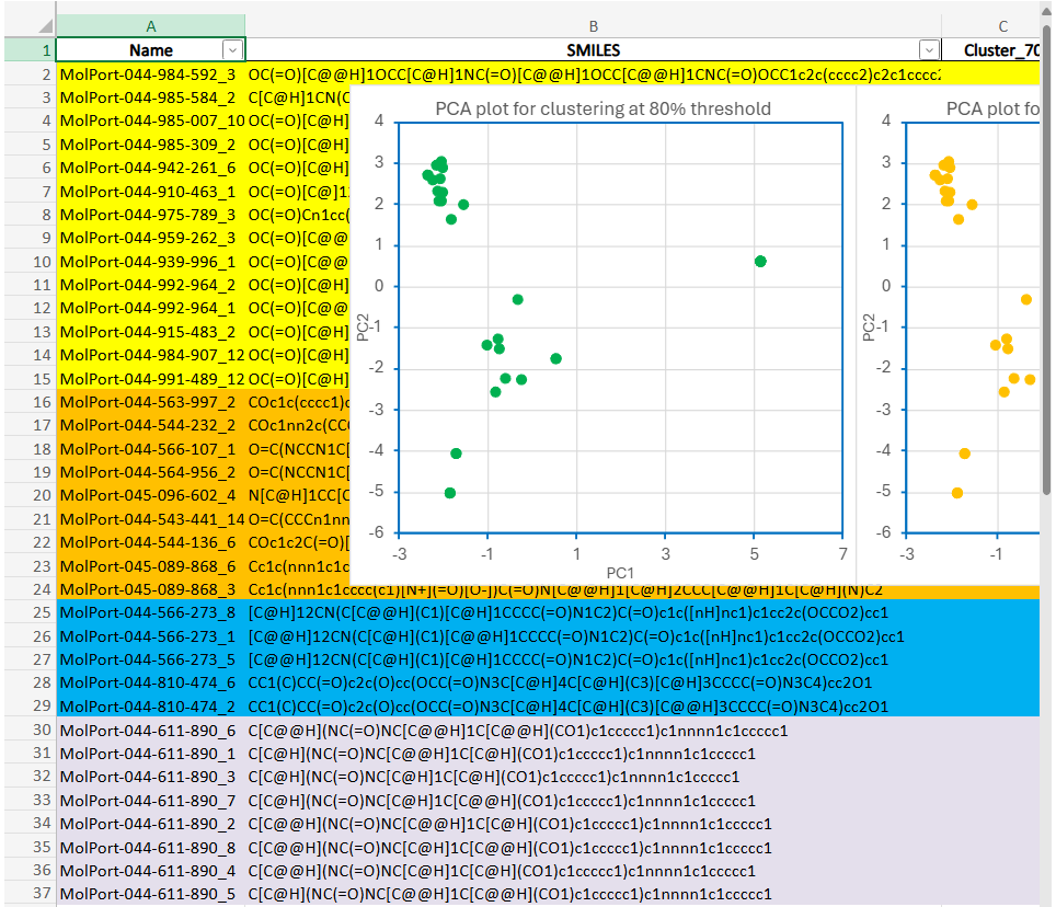
Finalmente una nueva versión del script de Python que genera los gráficos PCA con circulos que señalan los clusters de clusters y un fichero Excel con todos los datos.
import pandas as pd
import numpy as np
import matplotlib.pyplot as plt
import seaborn as sns
import os
from rdkit import Chem
from rdkit.Chem import DataStructs
from rdkit.Chem.rdFingerprintGenerator import GetMorganGenerator
from sklearn.cluster import AgglomerativeClustering, DBSCAN
from sklearn.decomposition import PCA
from scipy.spatial.distance import squareform
# === Configuración ===
input_file = r'd:\zzz\_buenos.txt'
output_folder = r'd:\zzz'
output_excel = os.path.join(output_folder, 'resultados_clusters.xlsx')
os.makedirs(output_folder, exist_ok=True)
# === Leer fichero ===
df_base = pd.read_csv(input_file, sep='\t')
names = df_base.iloc[:, 0].tolist()
smiles = df_base.iloc[:, 1].tolist()
# === Fingerprints ===
mol_list = [Chem.MolFromSmiles(s) for s in smiles]
generator = GetMorganGenerator(radius=2, fpSize=2048)
fps = [generator.GetFingerprint(m) for m in mol_list]
# === Matriz de distancia Tanimoto ===
def calc_distance_matrix(fps):
n = len(fps)
dist_mat = np.zeros((n, n))
for i in range(n):
for j in range(i + 1, n):
sim = DataStructs.TanimotoSimilarity(fps[i], fps[j])
dist = 1 - sim
dist_mat[i, j] = dist
dist_mat[j, i] = dist
return dist_mat
distance_matrix = calc_distance_matrix(fps)
fps_array = np.array([list(fp) for fp in fps], dtype=int)
# === DataFrame de resultados final ===
df_resultado = df_base.copy()
# === Thresholds de clustering ===
thresholds = [0.9, 0.8, 0.7]
for threshold in thresholds:
t_label = str(int(threshold * 100))
distance_threshold = 1 - threshold
# --- Clustering jerárquico ---
clustering = AgglomerativeClustering(
metric='precomputed',
linkage='complete',
distance_threshold=distance_threshold,
n_clusters=None
)
cluster_labels = clustering.fit_predict(distance_matrix)
df_resultado[f'Cluster_{t_label}'] = cluster_labels
# --- PCA ---
pca = PCA(n_components=2)
coords = pca.fit_transform(fps_array)
df_resultado[f'PCA_X_{t_label}'] = coords[:, 0]
df_resultado[f'PCA_Y_{t_label}'] = coords[:, 1]
# --- DBSCAN para superclusters ---
dbscan = DBSCAN(eps=1.5, min_samples=1)
superclusters = dbscan.fit_predict(coords)
df_resultado[f'Supercluster_{t_label}'] = superclusters
# --- Gráfico PCA + etiquetas + círculos ---
plt.figure(figsize=(10, 8))
palette = sns.color_palette("tab10", np.unique(superclusters).max() + 1)
sns.scatterplot(
x=coords[:, 0],
y=coords[:, 1],
hue=superclusters,
palette=palette,
legend='full',
s=60,
edgecolor='black'
)
# Añadir número de cluster jerárquico a cada punto
for i in range(len(coords)):
x, y = coords[i]
label = f'{cluster_labels[i]}'
plt.text(x + 0.1, y + 0.08, label, fontsize=10, color='black')
# Dibujar círculos rojos para cada supercluster
for sc_id in np.unique(superclusters):
indices = np.where(superclusters == sc_id)[0]
cluster_coords = coords[indices]
center_x = np.mean(cluster_coords[:, 0])
center_y = np.mean(cluster_coords[:, 1])
circle = plt.Circle((center_x, center_y), 1.5, color='red', fill=False, linewidth=2, linestyle='--')
plt.gca().add_patch(circle)
plt.text(center_x, center_y, f'C{sc_id}', color='red', ha='center', va='center', fontsize=10, weight='bold')
plt.title(f'PCA with Clusters and Superclusters (threshold {t_label}%)')
plt.xlabel('PC1')
plt.ylabel('PC2')
plt.legend(title='Supercluster', bbox_to_anchor=(1.05, 1), loc='upper left')
plt.tight_layout(rect=[0, 0, 0.85, 1])
# Guardar gráfico como PNG
fig_path = os.path.join(output_folder, f'pca_circles_{t_label}.png')
plt.savefig(fig_path, dpi=200)
plt.close()
print(f'✅ Imagen PCA guardada como: {fig_path}')
# === Guardar Excel final ===
df_resultado.to_excel(output_excel, index=False)
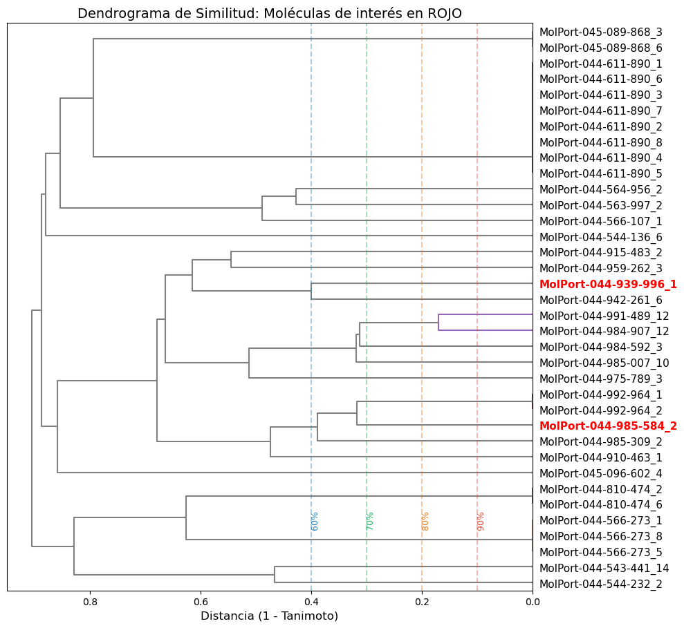
print(f'\n✅ Archivo Excel con todos los resultados guardado en: {output_excel}')Otra versión con opción de resaltar en rojo y negrita tus 'hits' y columna de nombres de cada molécula a la derecha.
import pandas as pd
import numpy as np
import matplotlib.pyplot as plt
from rdkit import Chem, DataStructs, RDLogger
from rdkit.Chem import AllChem
from scipy.cluster.hierarchy import dendrogram, linkage
from scipy.spatial.distance import pdist

# 1. Silenciar logs de RDKit (Deprecation Warnings, etc.)
RDLogger.DisableLog('rdApp.*')

# Configuración
file_path = r'C:\Users\jant\Desktop\notebook\smiles.txt'
# Tus moléculas de interés para resaltar
moleculas_interes = {'MolPort-044-985-584_2', 'MolPort-044-939-996_1'}

def get_data(path):
    try:
        # engine='python' y sep=None detecta automáticamente comas o tabs
        df = pd.read_csv(path, sep=None, engine='python')
        fps, names = [], []

        for _, row in df.iterrows():
            mol = Chem.MolFromSmiles(row['SMILES'])
            if mol:
                # ECFP4 (radio=2)
                fp = AllChem.GetMorganFingerprintAsBitVect(mol, radius=2, nBits=2048)
                # Convertir a array de bits
                arr = np.zeros((0,), dtype=np.int8)
                DataStructs.ConvertToNumpyArray(fp, arr)
                fps.append(arr)
                names.append(row['Name'])
        return np.array(fps), names
    except Exception as e:
        print(f"Error al procesar el archivo: {e}")
        return None, None

def plot_horizontal_highlighted_clusters(fps, names, target_list):
    # Cálculo de distancias (1 - Tanimoto) y Clustering
    dist_matrix = pdist(fps, metric='jaccard')
    # Método complete tiende a dar clusters más compactos
    Z = linkage(dist_matrix, method='complete')

    # Ajustar tamaño de figura, puede requerir más altura si hay muchas moléculas
    plt.figure(figsize=(10, len(names) * 0.2 + 2))

    # Crear el dendrograma HORIZONTAL
    dendro = dendrogram(
        Z,
        labels=names,
        orientation='left', # Girar 90 grados a la izquierda
        leaf_font_size=11,
        color_threshold=0.3, # Umbral de color para grupos >70% similar
        above_threshold_color='grey'
    )

    # --- MEJORA: Colorear etiquetas específicas en el eje Y (izquierda) ---
    ax = plt.gca()
    # Las etiquetas ahora están en el eje Y
    ylbls = ax.get_ymajorticklabels()

    for lbl in ylbls:
        # lbl.get_text() devuelve el nombre de la molécula
        if lbl.get_text() in target_list:
            lbl.set_color('red')
            lbl.set_weight('bold') # Resaltar en negrita
        else:
            lbl.set_color('black')

    # Líneas de referencia de Identidad (ahora verticales en el eje X)
    thresholds = {0.1: '90%', 0.2: '80%', 0.3: '70%', 0.4: '60%'}
    line_colors = ['#e74c3c', '#e67e22', '#27ae60', '#2980b9']

    for (dist, label), col in zip(thresholds.items(), line_colors):
        plt.axvline(x=dist, color=col, linestyle='--', alpha=0.4)
        # Etiqueta de texto para cada línea de referencia
        plt.text(dist, len(names) + 0.5, f' {label}', color=col, ha='left', va='bottom', rotation=90, fontsize=9)

    plt.title('Dendrograma de Similitud: Moléculas de interés en ROJO', fontsize=14)
    plt.xlabel('Distancia (1 - Tanimoto)', fontsize=12)
    # plt.ylabel('Nombres de las Moléculas', fontsize=12)
    plt.tight_layout()

    print(f"\n[INFO] Generando gráfico horizontal. Resaltando: {', '.join(target_list)}")
    plt.show()

if __name__ == "__main__":
    fps, names = get_data(file_path)
    if fps is not None and len(fps) > 1:
        plot_horizontal_highlighted_clusters(fps, names, moleculas_interes)
    else:
        print("No se encontraron suficientes moléculas para el análisis.")