Research → Frequency Distribution Analysis and Gaussian Fitting.

A Python script can be developed to run on Windows that reads a text file c:\bb\variable.txt containing a single column of numerical values and generates an output file c:\bb\distribución-de-frecuencias.txt with the frequency distribution (Y) of the variable for each bin (X). The script tabulates the data using relative frequencies expressed as percentages, allows the user to specify the bin width (e.g., 0.05), and defines the bin range according to the minimum and maximum values present in c:\bb\variable.txt.

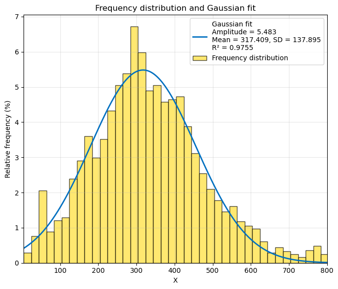
In addition, the script generates a bar histogram for visualization and performs a Gaussian fit of the calculated frequency distribution using the following equation:

In this expression, Amplitude corresponds to the height at the center of the distribution in Y-units, Mean represents the X-value at the center of the distribution, and SD is a measure of the distribution width, expressed in the same units as X.

The fitted Gaussian curve is superimposed on the histogram as an orange trend line. The calculated values of Amplitude, Mean, and SD are written to c:\bb\best-fit-values.txt. If the Gaussian fit is mathematically impossible, the file instead contains the message: "mathematically impossible fit".

import numpy as np
import matplotlib.pyplot as plt

# ==========================
# CONFIGURATION
# ==========================
INPUT_FILE = r"c:\bb\variable.txt"
OUTPUT_FREQ_FILE = r"c:\bb\frequency-distribution.txt"
OUTPUT_FIT_FILE = r"c:\bb\best-fit-values.txt"

BIN_WIDTH = 20
MAX_CONSOLE_BAR = 50

# ==========================
# DATA LOADING
# ==========================
data = np.loadtxt(INPUT_FILE)
data = data[np.isfinite(data)]

if data.size < 3:
    raise RuntimeError("Not enough data points.")

# ==========================
# BINNING
# ==========================
xmin, xmax = data.min(), data.max()
bins = np.arange(xmin, xmax + BIN_WIDTH, BIN_WIDTH)

counts, edges = np.histogram(data, bins=bins)
centers = 0.5 * (edges[:-1] + edges[1:])
total = counts.sum()

freq_percent = 100.0 * counts / total

# ==========================
# WRITE FREQUENCY TABLE
# ==========================
with open(OUTPUT_FREQ_FILE, "w", encoding="utf-8") as f:
    f.write("Bin_Center\tFrequency_%\n")
    for x, y in zip(centers, freq_percent):
        f.write(f"{x:.6f}\t{y:.6f}\n")

# ==========================
# CONSOLE HISTOGRAM
# ==========================
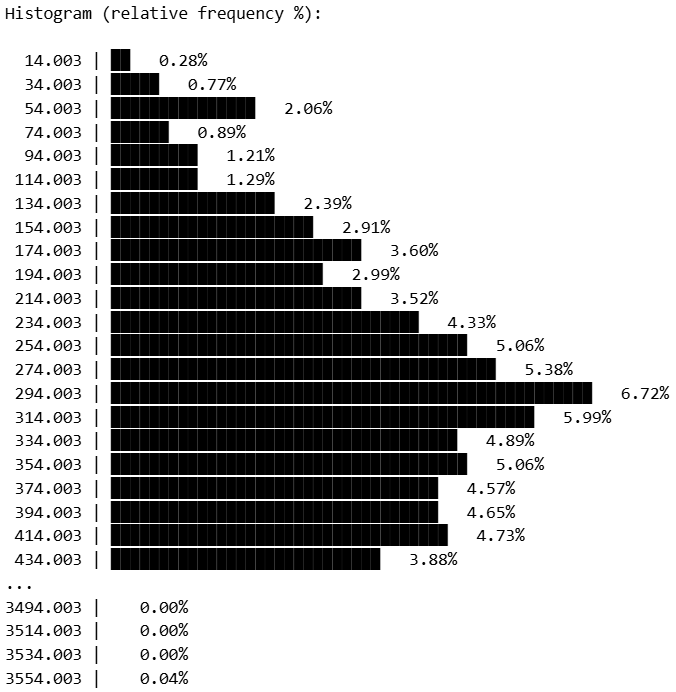
print("\nHistogram (relative frequency %):\n")

max_freq = freq_percent.max() if freq_percent.max() > 0 else 1.0

for x, y in zip(centers, freq_percent):
    bar_len = int((y / max_freq) * MAX_CONSOLE_BAR)
    bar = "█" * bar_len
    print(f"{x:8.3f} | {bar} {y:6.2f}%")

# ==========================
# GAUSSIAN MODEL
# ==========================
def gaussian(x, A, mu, sd):
    return A * np.exp(-0.5 * ((x - mu) / sd) ** 2)

fit_success = True

try:
    from scipy.optimize import curve_fit

    p0 = [
        freq_percent.max(),
        np.average(centers, weights=counts),
        np.std(data)
    ]

    popt, _ = curve_fit(
        gaussian,
        centers,
        freq_percent,
        p0=p0,
        maxfev=10000
    )

    A_fit, mu_fit, sd_fit = popt

    if sd_fit <= 0 or not np.isfinite(sd_fit):
        raise RuntimeError

    # ==========================
    # GOODNESS OF FIT
    # ==========================
    y_obs = freq_percent
    y_fit = gaussian(centers, A_fit, mu_fit, sd_fit)

    ss_res = np.sum((y_obs - y_fit) ** 2)
    ss_tot = np.sum((y_obs - np.mean(y_obs)) ** 2)

    R2 = 1.0 - ss_res / ss_tot if ss_tot > 0 else np.nan

    # Chi-square (assuming Poisson statistics in percentage space)
    sigma = np.sqrt(np.maximum(y_obs, 1e-6))
    chi2 = np.sum(((y_obs - y_fit) / sigma) ** 2)
    dof = len(y_obs) - 3
    chi2_red = chi2 / dof if dof > 0 else np.nan

except Exception:
    fit_success = False

# ==========================
# WRITE FIT RESULTS
# ==========================
with open(OUTPUT_FIT_FILE, "w", encoding="utf-8") as f:
    if fit_success:
        f.write(f"Amplitude = {A_fit:.6f}\n")
        f.write(f"Mean = {mu_fit:.6f}\n")
        f.write(f"SD = {sd_fit:.6f}\n")
        f.write(f"R_squared = {R2:.6f}\n")
        f.write(f"Reduced_chi_squared = {chi2_red:.6f}\n")
    else:
        f.write("mathematically impossible fit\n")

# ==========================
# PLOT
# ==========================
plt.figure(figsize=(7, 6))

plt.bar(
    centers,
    freq_percent,
    width=BIN_WIDTH,
    color="#FFDF33",
    edgecolor="black",
    alpha=0.7,
    label="Frequency distribution"
)

if fit_success:
    # Define plotting range based on Gaussian support (±3.5 SD)
    x_left = max(xmin, mu_fit - 3.5 * sd_fit)
    x_right = min(xmax, mu_fit + 3.5 * sd_fit)

    x_fit = np.linspace(x_left, x_right, 1000)
    y_fit_curve = gaussian(x_fit, A_fit, mu_fit, sd_fit)

    label = (
        f"Gaussian fit\n"
        f"Amplitude = {A_fit:.3f}\n"
        f"Mean = {mu_fit:.3f}, SD = {sd_fit:.3f}\n"
        f"R² = {R2:.4f}"
    )

    plt.plot(
        x_fit,
        y_fit_curve,
        color="#0070C0",
        linewidth=2,
        label=label
    )

    plt.xlim(x_left, x_right)

plt.xlabel("X")
plt.ylabel("Relative frequency (%)")
plt.title("Frequency distribution and Gaussian fit")
plt.legend()
plt.grid(alpha=0.3)
plt.tight_layout()
plt.show()

Text file example: c:\bb\variable.txt

---